Fits a user-defined nonlinear model to each bottle in a rumen_gp dataset.
Value
A custom_fit object containing:
Model name
Formula
Starting values
Parameter bounds
Parameter estimates
Model diagnostics
Predicted values
Residuals
Details
Overview
This function allows researchers to fit
custom nonlinear kinetic equations using
minpack.lm::nlsLM().
Custom models integrate directly with:
making them fully compatible with the rumenGP modeling framework.
Formula Requirements
The model formula must:
Use
Gas_mLas the response variableUse
Time_has the time variableInclude all parameters listed in
start
Example:
Gas_mL ~
  A *
  (
    Time_h /
    (
      Time_h + K
    )
  )
Starting Values
Starting values are supplied through
start.
Example:
start = list(
  A = 150,
  K = 10
)
Good starting values often improve convergence and reduce fitting failures.
Examples
files <- example_data()
raw_data <- read_ankom(
files$ankom
)
metadata <- read_metadata(
files$metadata
)
gp <- process_ankom(
raw_data,
metadata,
headspace_ml = 210,
temperature_c = 39
)
# Hyperbolic model
custom_fit <- fit_custom(
data = gp,
formula =
Gas_mL ~
A *
(
Time_h /
(
Time_h + K
)
),
start = list(
A = 150,
K = 10
),
lower = c(
A = 0,
K = 0
),
model_name = "Hyperbolic"
)
#> Warning: Large negative pressure values detected. Minimum PSI = -1.274 . Please inspect the affected bottles.
#> rumenGP data validation passed.
#> Observations: 1752
#> Heads: 24
#> Treatments: 5
summary(custom_fit)
#>
#> Custom model summary
#> --------------------
#> Model name: Hyperbolic
#>
#> Formula:
#> Gas_mL ~ A * (Time_h/(Time_h + K))
#>
#> Total bottles: 24
#> Successful fits: 23
#> Failed fits: 1
#> Mean R-squared: 0.8911
#> Mean RMSE: 3.6575
#> Mean AIC: 393.3084
#> Mean BIC: 400.1798
#>
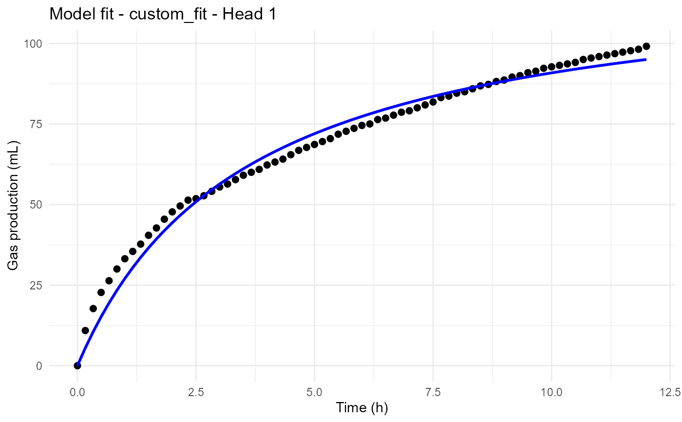
plot_fit(
custom_fit,
head = 1
)
 plot_residuals(
custom_fit,
head = 1
)
#> `geom_smooth()` using formula = 'y ~ x'
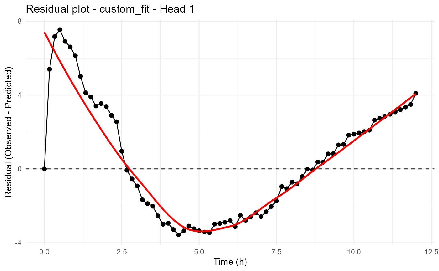
plot_residuals(
custom_fit,
head = 1
)
#> `geom_smooth()` using formula = 'y ~ x'
 # Compare with built-in models
compare_models(
Groot = fit_groot(gp),
Hyperbolic = custom_fit
)
#> Warning: Large negative pressure values detected. Minimum PSI = -1.274 . Please inspect the affected bottles.
#> rumenGP data validation passed.
#> Observations: 1752
#> Heads: 24
#> Treatments: 5
#> Model Bottles Successful_Fits Failed_Fits Mean_R2 Mean_RMSE Mean_RSS
#> 1 Groot 24 23 1 0.9768621 2.230506 518.1984
#> 2 Hyperbolic 24 23 1 0.8911079 3.657539 1108.4600
#> Mean_AIC Mean_BIC Lambda_Boundary
#> 1 302.3719 311.4785 0
#> 2 393.3084 400.1798 0
# Compare with built-in models
compare_models(
Groot = fit_groot(gp),
Hyperbolic = custom_fit
)
#> Warning: Large negative pressure values detected. Minimum PSI = -1.274 . Please inspect the affected bottles.
#> rumenGP data validation passed.
#> Observations: 1752
#> Heads: 24
#> Treatments: 5
#> Model Bottles Successful_Fits Failed_Fits Mean_R2 Mean_RMSE Mean_RSS
#> 1 Groot 24 23 1 0.9768621 2.230506 518.1984
#> 2 Hyperbolic 24 23 1 0.8911079 3.657539 1108.4600
#> Mean_AIC Mean_BIC Lambda_Boundary
#> 1 302.3719 311.4785 0
#> 2 393.3084 400.1798 0