Compare Residuals Across Models

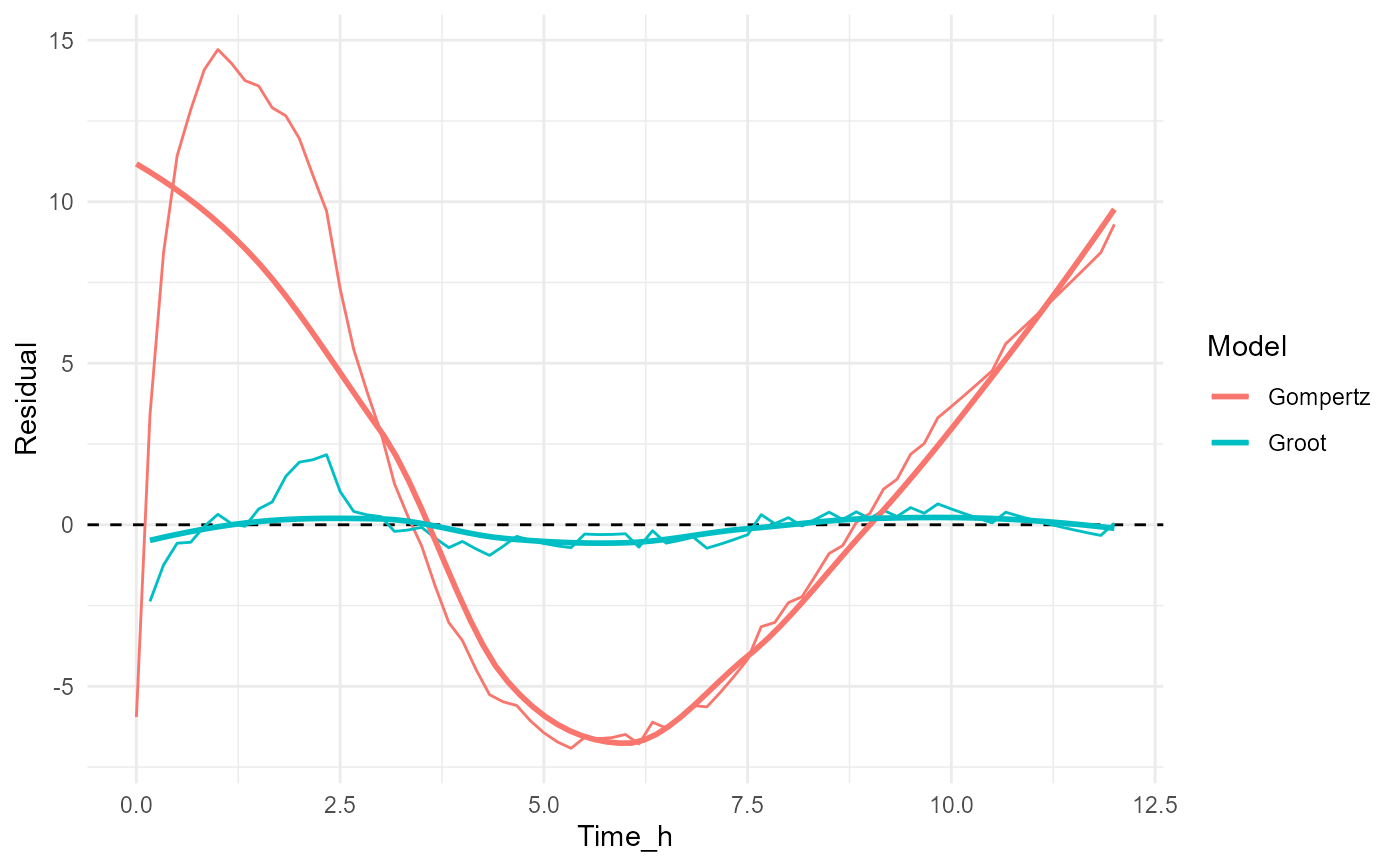
Displays residuals from multiple fitted models for a selected bottle.

Usage

plot_residual_comparison(..., head)

Arguments

...

Fitted model objects.

head

Head identifier.

Value

A ggplot2 object.

Details

Residuals are calculated as:

$$ Observed - Predicted $$

and can be used to evaluate:

• Model bias

• Systematic prediction errors

• Heteroscedasticity

• Relative model performance

Models with residuals that are randomly distributed around zero are generally preferred over models showing systematic patterns.

See also

plot_residuals, plot_model_comparison, compare_models, fit_groot, fit_gompertz

Examples

files <- example_data()

raw_data <- read_ankom(
  files$ankom
)

metadata <- read_metadata(
  files$metadata
)

gp <- process_ankom(
  raw_data,
  metadata,
  headspace_ml = 210,
  temperature_c = 39
)

groot_fit <- fit_groot(
  gp
)
#> Warning: Large negative pressure values detected. Minimum PSI = -1.274 . Please inspect the affected bottles.
#> rumenGP data validation passed.
#> Observations: 1752
#> Heads: 24
#> Treatments: 5

gompertz_fit <- fit_gompertz(
  gp
)
#> Warning: Large negative pressure values detected. Minimum PSI = -1.274 . Please inspect the affected bottles.
#> rumenGP data validation passed.
#> Observations: 1752
#> Heads: 24
#> Treatments: 5

plot_residual_comparison(
  Groot = groot_fit,
  Gompertz = gompertz_fit,
  head = 1
)
#> `geom_smooth()` using formula = 'y ~ x'